Epigenetics applications with Omni-C¶

In this section you will learn how to:

Identify Topologically Associated Domains (TADs)
Identify A/B compartments

Identify Topologically Associated Domains (TADs)¶

The .hic file that you generated can be used for identifying Topologically Associated Domains (TADs) in the contact map using the arrowhead utility of Juicer Tools

Parameter	Function
-Xmx	The flag Xmx specifies the maximum memory allocation pool for a Java virtual machine, from our experience 48000m works well when processing human data sets. If you are not sure how much memory your system has, run the command `free -h` and check the value under total.
Djava.awt.headless=true	Java is ran in a headless mode when the application does not interact with a user (if not specified, the default is Djava.awt.headless=false)
arrowhead	The arrowhead command is used to identify contact domains along the diagonal
--threads	Specifies the numbers of threads to be used (integer number)
-k	Normalization to be used. KR (Knight-Ruiz) balancing is recommended (other avilable normalization methods are VC and VC_SQRT or NONE, (this is not recommended)
-m	Size of the sliding window along the diagonal in which contact domains will be found. Must be an even number as (m/2) is used as the increment for the sliding window. Recommended value: 2000 (this is also the default)
-r	Resolution for which Arrowhead will be run. We recommend running with various resolutions, e.g.: 5kB (5000), 10kB (10000), 25kb (25000) and 50kb (50000). The quality of the results at the various resolutions is highly dependent on the depth of sequencing
*.hic	hic input file, containing the contact matrix
output directory	a path to the directory in which a bedpe file containing the contact domains will be saved (the name of the file is composed of the resolution followed by _blocks.bedpe). The bedpe file, is a text file with 16 fields in each row. For more details on the file format, see the table below

Command:

java -jar -Xmx<memory> -Djava.awt.headless=true -jar <path_to_juicer_tools.jar> arrowhead --threads <no_of_threads> -k <normalization_type> -m <sliding_window> -r <resolution> <*.hic> <output_path>

Example:

java -jar -Xmx48000m  -Djava.awt.headless=true -jar ./Omni-C/juicer_tools.jar arrowhead --threads 16 -k KR -m 2000 -r 10000 contact_map.hic TAD_calls

The above command will result in a new file “10000_blocks.bedpe” inside the “TAD_calls” directory.

The bedpe output file will contain a list of contact domains with the following 16-field header:

chr1 x1 x2 chr2  y1 y2 name  score strand1  strand2  color score uVarScore   lVarScore   upSign   loSign

Field	Description
chr1/chr2	The chromosome that the domain is located on
x1,x2/y1,y2	The interval spanned by the domain (contact domains manifest as squares on the diagonal of a Hi-C matrix and as such: x1=y1, x2=y2)
name	typically this field is empty (contains “.”)
score	typically this field is empty (contains “.”)
strand1	typically this field is empty (contains “.”)
strand2	typically this field is empty (contains “.”)
color	The color that the feature will be rendered as if loaded in Juicebox
score	The corner score, a score indicating the likelihood that a pixel is at the corner of a contact domain. Higher values indicate a greater likelihood of being at the corner of a domain
uVarScore	The variance of the upper triangle
lVarScore	The variance of the lower triangle
upSign	-1*(sum of the sign of the entries in the upper triangle)
loSign	Sum of the sign of the entries in the lower triangle

Principle component of the contact matrix¶

The contact matrix .hic can also be used for calculating the Pearson’s correlation matrix of the Observed/Expected for intra-chromosomal contacts. The eigenvector is the first principal component of the Pearson’s matrix and it implies on the compartmentalization of the DNA at high level. The sign of the eigenvector typically indicates the compartment type A/B (active/inactive).

The Principle component of the contact matrix can be calculated using the eigenvector utility of Juicer Tools

Parameter	Function
-Xmx	The flag Xmx specifies the maximum memory allocation pool for a Java virtual machine, from our experience 48000m works well when processing human data sets. If you are not sure how much memory your system has, run the command `free -h` and check the value under total.
Djava.awt.headless=true	Java is ran in a headless mode when the application does not interact with a user (if not specified, the default is Djava.awt.headless=false)
eigenvector	The eigenvector command is used to calculate the first principal component of the Pearson’s Observed/Expected matrix
-p	Optional, force with curren parameters. When running with resolution < 500kb this may take very long time and by default the run will be canceled (output file will be empty). To force the run with any resolution < 500kb use the -p flag
VC/VC_SQRT/KR	Normalization to be used. KR (Knight-Ruiz) balancing is recommended.
*.hic	hic input file, containing the contact matrix
chr	The chromosome for which the principle component will be calculated (make sure that same format as in the reference is used, e.g. chrX or x, depending on the reference)
output directory	a path to the directory in which a bedpe file containing the contact domains will be saved (the name of the file is composed of the resolution followed by _blocks.bedpe). The bedpe file, is a text file with 16 fields in each row. For more details on the file format, see the table below
BP	resolution type (FRAG is another resolution type, this option is not covered in this documentation)
Resolution	Which resolution to be used for the calculation (integer). Since the goal here is to identify high level compartments 1M (100000) or 500k (500000) are typically sufficient
Output file	Name of text file for recording the calculated values. The output is a list of eigenvalues recorede for each bin, sorted by order on the chromosome. E.g. if the chromosome lenght 43Mb and a bin size of 1000000 was used, the output will be a list of 43 eigenvalues in text format.

Command:

java -jar -Xmx<memory>  -Djava.awt.headless=true -jar <path_to_juicer_tools.jar> eigenvector <normalization_type> <*.hic> <chromosome> <resolution type> <resolution> <output file>

Example 1 (resolution >= 500kb):

java -jar -Xmx48000m  -Djava.awt.headless=true -jar ./Omni-C/juicer_tools.jar eigenvector KR contact_map.hic chr1 BP 1000000 PC_chr1.txt

Example 2 (resolution <= 500kb):

java -jar -Xmx48000m  -Djava.awt.headless=true -jar ./Omni-C/juicer_tools.jar eigenvector -p KR contact_map.hic chr1 BP 100000 PC_chr1.txt

As described in the table above, the output is a one columnn list of the eigenvalues as calculated for each one of the bins. For most of the common applications this format is not useful and we will guide you on how to convert it to more useful formats:

bedGraph format¶

To generate a bedgraph which details each bin interval followed by the associated eigenvalue you will generate a list of the bins intervals using the bedtools makewindows command and combine it with the output file of the previous step (juicer tools eigenvector).

Specify the chromosome of interest, first bp of the chromosome, last bp of the chromosome (you can find this information in the .genome file) in a tab delmitied format (as in a bed file format) and feed it to bedtools makewindows alongside the window size (same as the resolution used for juicer tools eigenvector). Finally, combine the two files using the paste command:

Command:

echo -e '<chromosome>\t<start position>\t<end position>'|bedtools makewindows -b stdin -w <window>|paste - <eigenvector output file> > <output.bedgraph>

Example:

echo -e 'chr1\t0\t248956422'|bedtools makewindows -b stdin -w 1000000|paste - PC_chr1.txt > PC_chr1.bedgraph

A/B compartments¶

Active regions in the genome were observed to have similar eigenvalues, the same is true for inactive regions. To identify the distinct compartments all the neighboring bins with same sign (>0 or <0) are merged into one region. In each chromosome all the regions with the same sign are classified as the same compartment type (A/B). Please note that the signs of PC values are arbitrary, to accurately assign compartment type to signs of PC values, you need knowledge beyond Omni-C data such as RNA-Seq, Methylation states, etc`

We will use the bedGraph file for generating a bedpe file containing the borders of the calculated A/B compartments:

bedtools allows merging of overlapping or neighboring (-d flag) intervals based on strandness (-s flag). We will use this utility by assigning + to all intervals with PC1 values >0 and - to all intervals with PC1 values <0 (A/B compartments has nothing to do with strandness, the + and - assignments are only from practical reasons for easy manupulation of the bed file). The strandness option assumes the strand information is on the 6th column, we will use the awk command to record + or - on the 6th column based on the PC values. Adjacent intervals with the same sign are merged together using bedtools merge Following merging, we will use the awk command to genetrate the final bedpe format.

Command:

awk '{if ($4 > 0) print $1"\t"$2"\t"$3"\t"".""\t"".""\t""+"; else if ($4 < 0) print $1"\t"$2"\t"$3"\t"".""\t"".""\t""-"}' <*.bedgraph>|bedtools merge -s -d 10  -c 6 -o distinct|awk '{print $1"\t"$2"\t"$3"\t"$1"\t"$2"\t"$3"\t"$4}'> <output.bedpe>

Example:

awk '{if ($4 > 0) print $1"\t"$2"\t"$3"\t"".""\t"".""\t""+"; else if ($4 < 0) print $1"\t"$2"\t"$3"\t"".""\t"".""\t""-"}' PC_chr1.bedgraph|bedtools merge -s -d 10  -c 6 -o distinct|awk '{print $1"\t"$2"\t"$3"\t"$1"\t"$2"\t"$3"\t"$4}'>chr1_AB.bedpe

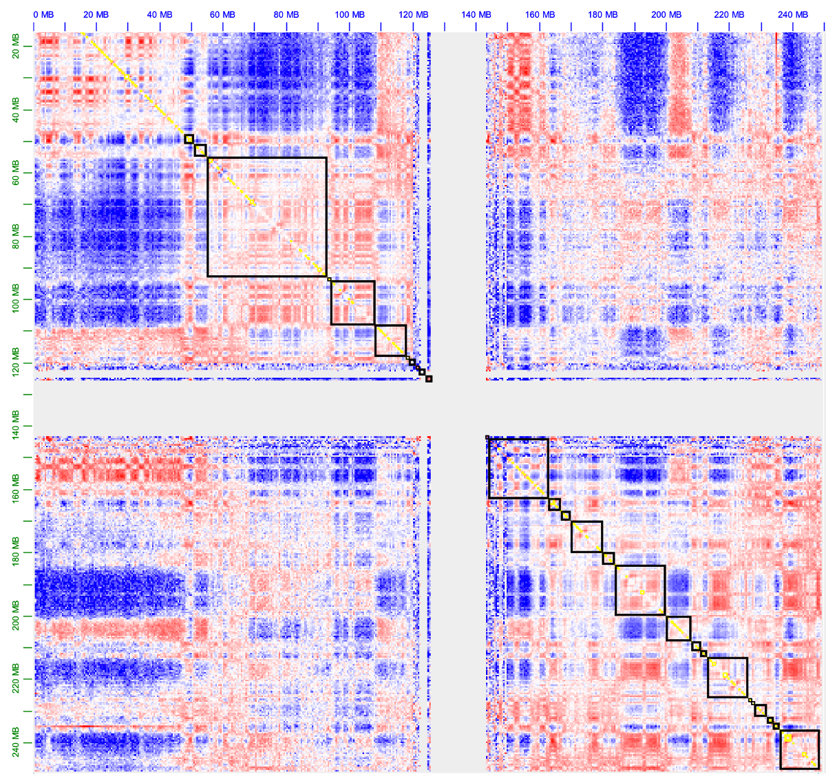
The figure below shows the observed/expected matrix of chr1 with the A/B compartments (black boxes) as generated with the commands above (visualized using Juicebox)